[1]:
%pylab inline
Populating the interactive namespace from numpy and matplotlib
VASP - Surface energy
In this example, we introduce how to perform VASP calculations using strucscan and calculate the formation energy of an example (100) fcc surface in Ni. This example requires two prerequisites: * a licensed VASP version * a configured resource directory including the necessary POTCAR for Ni
In the documentation, it is explained how to set up the resource directory for VASP. We will also need a settings template. For this, you can stick to the default one that comes with the repository. We will perform a spin-polarised calculation with an energy cut-off of 500 eV:
[2]:
! cat ../resources/engines/vasp/settings/500_SP.incar
! ISIF and IBRION flags will be set automatically by strucscan
ALGO            = Fast
PREC            = Accurate
EDIFF           = 1e-05
NSW             = 100
NELM            = 60
LREAL           = .FALSE.
LWAVE           = .FALSE.
ISPIN           = 2
LCHARG          = .FALSE.
LORBIT          = 11
ENCUT           = 500
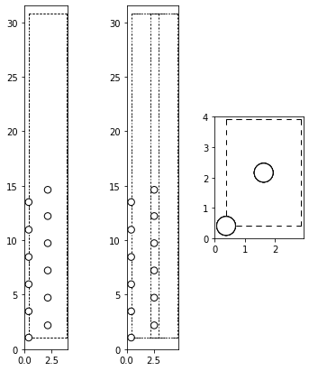
The structure
Let’s have a look at the surface structure that we want to investigate:
[3]:
from ase.visualize.plot import plot_atoms
from ase import io

structname = "../structures/unaries/surfaces/fcc_110surf_12at.cfg"
atoms = io.read(structname, format="cfg")

fig, axs = plt.subplots(1, 3, figsize=(6,7))
for ind, rotation in enumerate(['90x,90y', '90x,45y', '0x']):
    plot_atoms(atoms, rotation=(rotation), ax=axs[ind])
plt.show()
The input dictionary
The next step is to set up the input dictionary properly. We can either start from scratch as in the previous example or start right away with the pre-implemented example for vasp:
[4]:
from strucscan.resources.inputyaml import *
input_dict = VASP().EXAMPLE
input_dict
[4]:
{'species': 'Ni Al_pv',
 'engine': 'VASP 5.4',
 'machine': 'example_vasp',
 'ncores': '1',
 'nnodes': '1',
 'queuename': 'none',
 'potential': 'PBE',
 'properties': 'atomic',
 'prototypes': 'L1_2',
 'settings': '500_SP.incar',
 'magnetic configuration': 'SP',
 'initial magnetic moments': '2.0 0.',
 'kdens': '0.15',
 'kmesh': 'Monkhorst-pack',
 'initial atvolume': 'default',
 'verbose': False,
 'monitor': True,
 'submit': True,
 'collect': False}
The example input is already configured for our example machine vasp_example which features no queueing system but we need to adapt some values:
[5]:
input_dict.update({"species": "Ni",
                   "potentials": "PBE",
                   "properties": "atomic",
                   "prototypes": "fcc.cfg fcc_110surf_12at.cfg",
                   "initial magnetic moments": "2.0",
                   "kdens": "0.15",
                   "verbose": True})
input_dict
[5]:
{'species': 'Ni',
 'engine': 'VASP 5.4',
 'machine': 'example_vasp',
 'ncores': '1',
 'nnodes': '1',
 'queuename': 'none',
 'potential': 'PBE',
 'properties': 'atomic',
 'prototypes': 'fcc.cfg fcc_110surf_12at.cfg',
 'settings': '500_SP.incar',
 'magnetic configuration': 'SP',
 'initial magnetic moments': '2.0',
 'kdens': '0.15',
 'kmesh': 'Monkhorst-pack',
 'initial atvolume': 'default',
 'verbose': True,
 'monitor': True,
 'submit': True,
 'collect': False,
 'potentials': 'PBE'}
Please note that you may want to adapt the machine config.yaml to the machine on which you are running VASP. In this example, the config.yaml looks as following:
[6]:
from pprint import pprint
import yaml
with open("../resources/machineconfig/example_vasp/config.yaml", "r") as stream:
        config = yaml.safe_load(stream)
pprint(config)
{'VASP': {'serial': 'module load vasp/5.4.4\nvasp_std\n'},
 'scheduler': 'noqueue',
 'smallest queue': None}
We also added fcc.cfg to our list of prototypes. This is the reference structure that we need to calculate the formation energy. Now, we can get started: ## Running strucscan
[ ]:
from strucscan.core.jobmanager import JobManager

JobManager(input_dict)
Data tree path:                /home/users/pietki8q/git/strucscan-master/data
Structure repository:          /home/users/pietki8q/git/strucscan-master/structures
Resource repository:           /home/users/pietki8q/git/strucscan-master/resources

Optional key 'k points file' not provided. Default value will be used: (None)


key:                           : your input                                         what strucscan reads
----------------------------------------------------------------------------------------------------
species                        : Ni                                                 Ni
engine                         : VASP 5.4                                           VASP 5.4
machine                        : example_vasp                                       example_vasp
ncores                         : 1                                                  1
nnodes                         : 1                                                  1
queuename                      : none                                               none
potential                      : PBE                                                PBE
properties                     : atomic                                             atomic
prototypes                     : fcc.cfg fcc_110surf_12at.cfg                       fcc.cfg fcc_110surf_12at.cfg
settings                       : 500_SP.incar                                       500_SP.incar
magnetic configuration         : SP                                                 SP
initial magnetic moments       : 2.0                                                2.0
kdens                          : 0.15                                               0.15
kmesh                          : Monkhorst-pack                                     Monkhorst-pack
initial atvolume               : default                                            default
verbose                        : True                                               True
monitor                        : True                                               True
submit                         : True                                               True
collect                        : False                                              False
potentials                     : PBE                                                PBE
k points file                  : (not set)                                          (not set)

>> Initializing:
Initialized  Ni atomic
Initialized  Ni atomic
Initialized  Ni atomic

2 jobs in JobList:
------------------------------------------------------------------------------------------------------------------
  #: jobpath                                                       prototype path
------------------------------------------------------------------------------------------------------------------
  0: VASP_5_4__500_kdens_0_150_SP_PBE/Ni/atomic__fcc_110surf_12at__Ni12  unaries/surfaces/fcc_110surf_12at.cfg
  1: VASP_5_4__500_kdens_0_150_SP_PBE/Ni/atomic__fcc__Ni           unaries/bulk/fcc.cfg

  #: jobpath                                                      id       status   start                end
------------------------------------------------------------------------------------------------------------------
  0 VASP_5_4__500_kdens_0_150_SP_PBE/Ni/atomic__fcc_110surf_12at__Ni12 None     does not exist
  1 VASP_5_4__500_kdens_0_150_SP_PBE/Ni/atomic__fcc__Ni          None     does not exist


>> Entering loop:
Determining surface energy
After finishing successfully, strucscan saves the data from the calculation in dictionaries in a human-readable JSON format.
[ ]:
! ls ../data/VASP_5_4__500_kdens_0_150_SP_PBE/
[ ]:
import json

with open("../../VASP_5_4__500_kdens_0_150_SP_PBE__Ni__output_dict.yaml") as stream:
    output_dict = json.load(stream)
    stream.close()

from pprint import pprint
pprint(output_dict)
In order to calculate the surface energy with the following equation, we also need to determine the surface area A:
For this, we need to read the final surface structure manually.
[9]:
from ase import io

surface_atoms = io.read("../../data/VASP_5_4__500_kdens_0_150_SP_PBE/Ni/atomic__fcc_110surf_12at__Ni12/OUTCAR.gz", format="vasp-out")
surface_atoms
[9]:
Atoms(symbols='Ni12', pbc=True, cell=[1.978349761, 2.797335995, 23.740192654], calculator=SinglePointDFTCalculator(...))
[11]:
eV_A2_to_mJ_m2 = 1.60218e-19 * 1e20 * 1e3

surface_structure_energy = output_dict["atomic__fcc_110surf_12at__Ni12"]["structure_energy"]
surface_n_at = output_dict["atomic__fcc_110surf_12at__Ni12"]["n_atom"]
surface_area = np.linalg.det(surface_atoms.get_cell()[:2, :2])

basis_ref_energy = output_dict["atomic__fcc__Ni"]["structure_energy"]
basis_ref_n_atom = output_dict["atomic__fcc__Ni"]["n_atom"]

surface_formation_energy = (surface_structure_energy / surface_n_at - basis_ref_energy / basis_ref_n_atom) / (2 * surface_area)
print(surface_formation_energy * eV_A2_to_mJ_m2)
1379.5079416851156
[ ]: